My interest in GDBs grew out of my management consulting work and a recent presentation I gave at a media ecology conference (Cheyunski 2016). While preparing my presentation, I learned of an organizational modeling tool with a GDB foundation (Concentra Analytics n.d.). It occurred to me that a GDB could provide an effective way to model and analyze the personal/organizational storylines and media forces I was investigating. However, because my focus has been on people issues and not programming, I realized that I had to learn GDB fundamentals first. Since my focus was on method not scale, I chose to work with a small set of data for my initial GDB learning.
Because I saw examples in YouTube GDB tutorials utilizing books, I decided to use my own book data. Moreover, it seemed that I could later create a GDB to examine the relationships among books I was reading pertaining to my evolving, more eclectic management and media ecology interests. For example, what are emerging new media approaches in analytics, modeling, simulation, and visualization? What are the origins of these methods? Where are they being applied? In what ways do these efforts relate and what are their implications? How can these approaches be further used with benefit in different areas of inquiry?
From these activities, I have derived the following 10-step learning guide for beginners, i.e. non-programmers, who are either curious or interested in learning about GDBs. This guide provides a sequential blueprint for students and teachers to follow to develop GDB capabilities for enhancing their research and studies. By following this ten-step guide, one can start to learn and construct a small-scale GDB as a stepping stone for more complex modeling and analysis of larger scale networked information.
To begin to learn GDBs, non-programmers such as myself have needed to become familiar with a GDB application. There are other data visualization programs including Gephi, Cytoscape, or Palladio that have been used in the humanities (Brooks 2017) and elsewhere or even within different GDB applications (Xu 2018). Gephi is geared more toward massive network data visualizations such as content within The New York Times, for example, or Twitter traffic. Cytoscape was originally designed for biological research, and now acts as a general platform for complex network and graphic analysis. Palladio is a specialized application for graphing historical analysis in documentation such as Galileo’s or Luther’s correspondence as part of The Republic of Letters or the Grand Tour. While these programs have their strengths, GDBs allow one to start with rudimentary data and develop a simple data model that can then be expanded, revised, and scaled up as desired, particularly for discovery where initial questions are broad and require further clarification and refinement. Learners should consider whether one of the other programs might be more suited to their needs (e.g. if they just wanted to make a visualization of information that clearly fits well within an already existing data model). However, GDBs seem to provide the most flexibility and options in evolving models for new or enhanced exploration and investigation.
Among the various prominent GDB applications, I found that Neo4j is readily accessible with extensive supporting information along with training videos available and updates extending its features and reach. For instance, at one point, Neo4j added plugins for Gephi and Cytoscape to allow people to take advantage of the graphics in the respective programs (e.g. see Villedieu 2014). Because of its relative ease of use and possibilities for analysis, I chose to concentrate on Neo4j.
In this tutorial, I will use my Sample Book and Review Data as shown in Table 1. I found that using familiar subject matter made learning more natural and relevant. This dataset includes information on 15 of the books I have read and the related reviews I have written in recent years. In putting together, the Sample Booklist and Review Data for this article, I had the following questions: How could titles in my Sample Booklist and Review Data best pertain or illuminate GDBs and their potential utilization? What could defining their relationships reveal about the titles included and GDB use? How could this smaller manageable Sample Booklist and Review set be considered to demonstrate utilizations with a wider set?
Neo4j and other GDBs can be used with all kinds of data and situations, so learners can think about types of data that would be more pertinent for them as they continue with the ten steps. For example, they could think of later using their own annotated booklist, a dissertation bibliography, or perhaps mapping key author books against other references. Thus, one can easily imagine an aspiring humanities scholar’s thesis that includes GDB visuals.
This guide was created by me, a GDB novice, for others who are new to GDBs. I also recommend consulting tutorials on YouTube and the graph database entry on Wikipedia.
Step 1: Become acquainted with fundamental GDB concepts and descriptive material about the Neo4j application
A graph database (GDB) shows data in nodes, properties, and relationships. In a GDB, data is represented in a network where significant objects (nodes), such as books, book reviews and their corresponding information (properties), are linked together directly (relationships), and can be readily depicted and retrieved. Within a more standard database, such as an Excel spreadsheet or relational database, the various cells need to be deliberately associated, defined, then extracted via formulas, functions, and manual effort. However, in a GDB, the different items that are included and represented by commands within the application can be conceptualized (become visual) and drawn as on a whiteboard (see Figure 1). Another advantage of GDBs is that this data model or data structure can be easily changed as one’s thinking evolves and relevant information expands.
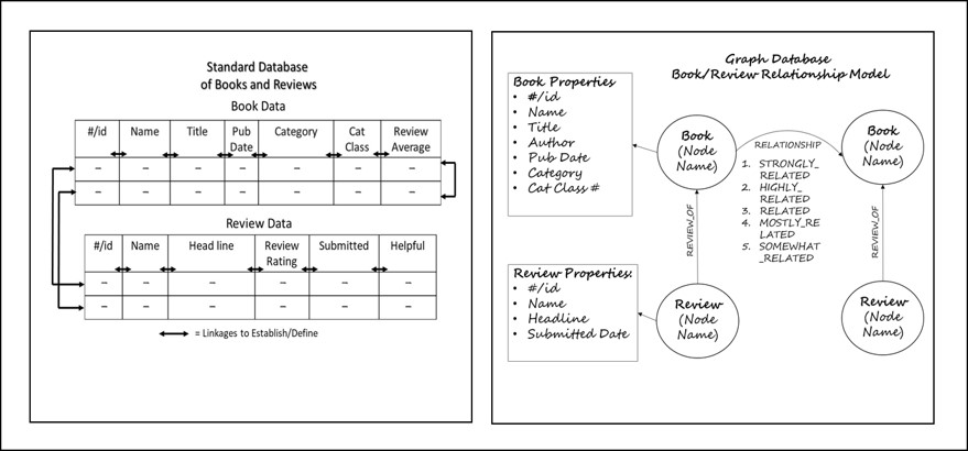
Figure 1. Standard vs. graph databases.
Step 2: Download Neo4j
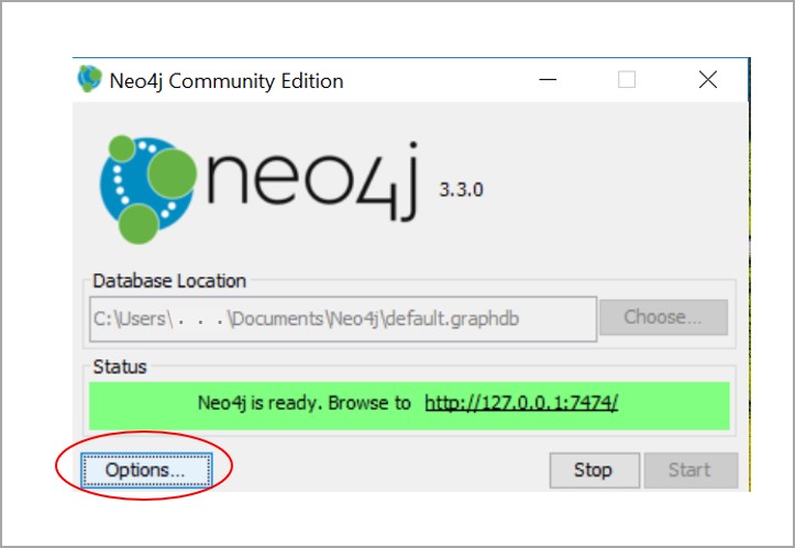
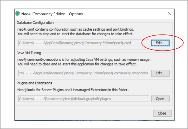
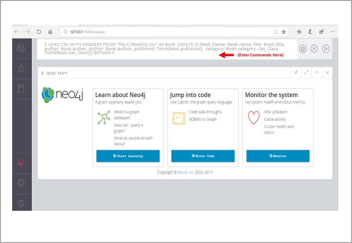
Users can access Neo4j via the GitHub website (https://github.com/neo4j/neo4j; see also Figure 2 for the particulars and the red arrow for the download).
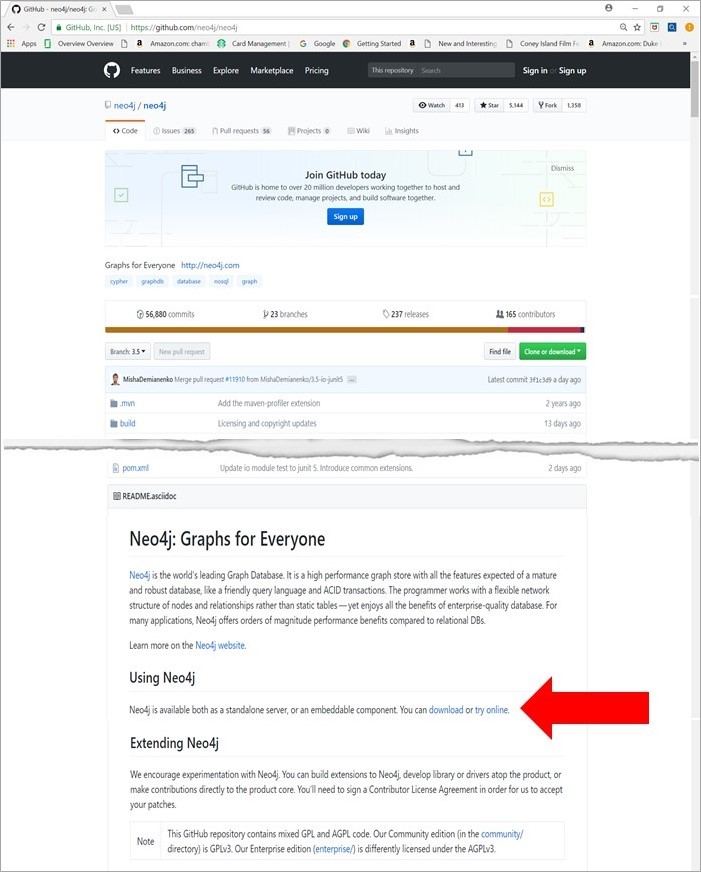
Figure 2. Neo4j download via GitHub.
Step 3:Become familiar with initial commands and create nodes in Neo4j
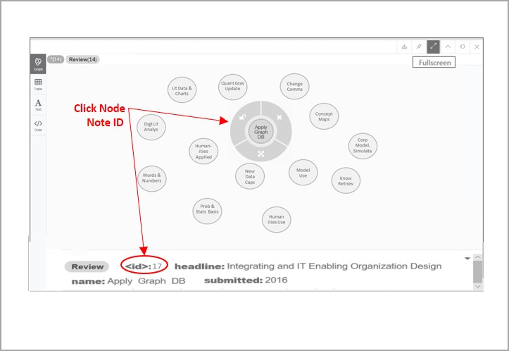
Enter a command manually in Neo4j with the booklist item to create the first node (see below and the red arrow in Figure 3):
| CREATE (x:Book{name:” Graph DBs”, title:” Graph Databases: New Opportunities for Connected Data, 2nd Edition”, author:”Ian Robinson”, Author:” Jim Webber”, published:2015, category:[“Computers & Technology”, “Databases & Big Data, Data Warehousing”], Cat_Class:600}) RETURN x |

Figure 3. Enter commands in Neo4j.
Next, enter the related review data in the same manner with the following command:
| CREATE (y:Review {name:”Good/ Hard Starter”, headline:[” Good Graph DB Starter Despite Challenges for Non-Programmers”], submitted:2017})RETURN y; |
After creating the nodes (where each one appears on screen), enter the following command to see the visual of both nodes together as shown in Figure 4:
| MATCH (n) RETURN n |
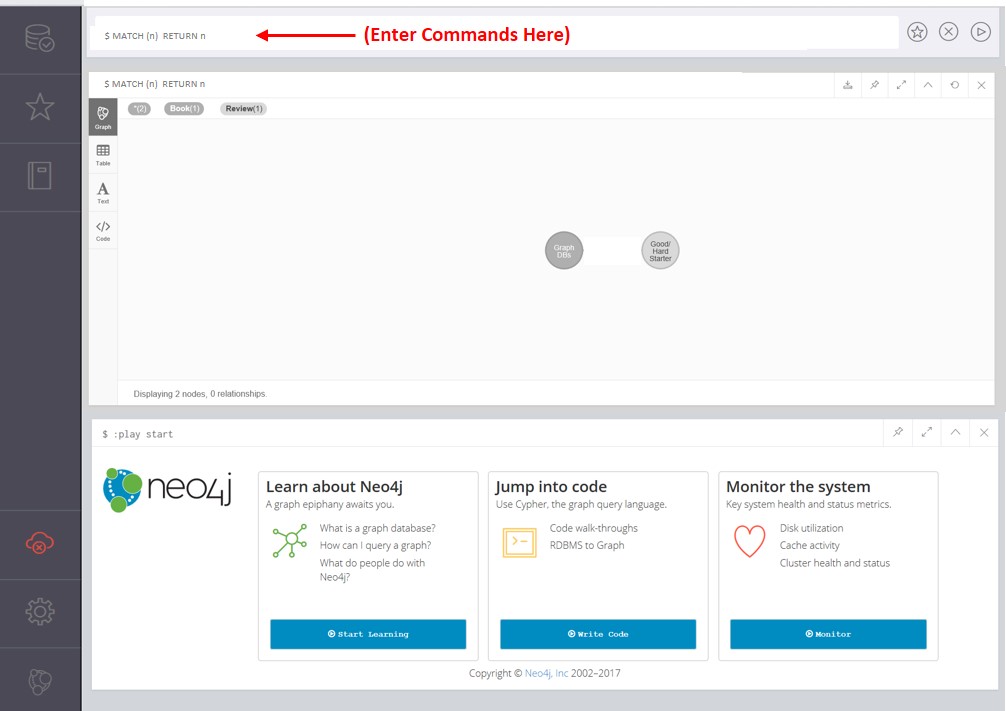
Figure 4. Book and review nodes.
Note that I use gray scale for my nodes in many of the Figures here. Later in the article, I show how you can use colors to assist with analyses.
Step 4: Repeat Step 3 to create nodes for the other items in the Sample Booklist and Review Data.
Note that all the information for this step for 14 other books and related review items is provided in Table 1 below. When originally working on my list, I began to get a sense of the diversity, or lack thereof, in my sources. Thus, for this set I chose to provide a fairly broad sample which is varied and seems pertinent to the objective of this article, i.e. creating and using GDBs.
Table 1. Sample Book & Review Data
| # | Book Node Name |
Title | Author | Author | Published | Category | Cat_ Class* | # | >Review Node Name | Headline | Submitted |
| 1 | Graph DBs | Graph Databases: New Opportunities for Connected Data, 2nd Edition | Ian Robinson | Jim Webber | 2015 | Computers & Technology, Databases & Big Data, Data Warehousing | 600 | 2 | Good/ Hard Starter | Good Graph DB Starter Despite Challenges for Non-Programmers | 2017 |
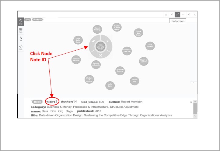
| 3 | Data Driv Org Dsgn | Data-driven Organization Design: Sustaining the Competitive Edge Through Organizational Analytics | Rupert Morrison | 2015 | Business & Money, Processes & Infrastructure, Structural Adjustment | 600 | 4 | Apply Graph DB | Integrating and IT Enabling Organization Design | 2016 | |
| 5 | Theory of Comms | Theories of Communication | Eric McLuhan | Marshall McLuhan | 2011 | Textbooks, Communication & Journalism, Communications | 300 | 6 | Change Comms | McLuhan and the Classical Art of Rhetoric (“Change Communica-tion”) Revealed | 2012 |
| 7 | Secr Knowldg | Secret Knowledge: Rediscovering the Lost Techniques of the Old Masters (Expanded) | David Hockney | 2006 | Arts & Photography, Painting, Oil Painting | 700 | 8 | Know Retriev | First Rate Lessons in “Secret Knowledge” Retrieval | 2014 | |
| 9 | Create Use Knowledge | Learning, Creating, and Using Knowledge: Concept Maps as Facilitative Tools in Schools and Corporations | Joseph D. Novak | 2009 | Education & Teaching, Schools & Teaching, Computers & Technology | 300 | 10 | Concept Maps | Concept Mapping’s Origins, Rationale, Theory, and Application | 2014 | |
| 11 | Keep Up w Quants | Keeping Up with the Quants: Your Guide to Understanding and Using Analytics | Thomas H. Davenport | Jinho Kim | 2013 | Business & Money, Education & Reference, Statistics | 300 | 12 | New Data Caps | Understanding/ Learning to Utilize New Data/Analytic Capabilities | 2015 |
| 13 | Remodel Comms | Remodelling Communication: From WWII to the WWW | Gary Genosko | 2013 | Politics & Social Sciences, Social Sciences, Communication & Media Studies | 300 | 14 | Model Use | Appreciation of Different Model and Communication Dimensions | 2015 | |
| 15 | Serious Play | Serious Play: How the World’s Best Companies Simulate to Innovate | Michael Schrage | 1999 | Science & Math, Technology, History of Technology | 600 | 16 | Corp Model, Simulate | Continues to Offer Rationale/ Implications Regarding Modeling and Simulation | 2015 | |
| 17 | Distant Reading | Distant Reading | Franco Moretti | 2013 | Literature & Fiction, History & Criticism, Comparative Literature | 800 | 18 | Lit Data & Charts | Valuable Examples of Data, Chart and Graph Use to Analyze Literature | 2016 | |
| 19 | Unfin Game | The Unfinished Game: Pascal, Fermat, and the Seventeenth-Century Letter that Made the World Modern | Keith Devlin | 2010 | Science & Math, Mathematics, History | 500 | 20 | Prob & Stats Basis | Basis of Probability/Statistics for Our Modern World and Limitations | 2016 | |
| 21 | Best Seller Code | The Bestseller Code: Anatomy of the Blockbuster Novel | Jodie Archer | Matthew L. Jockers | 2016 | Literature & Fiction, History & Criticism, Books & Reading | 800 | 22 | Digt Lit Analys | Popularizing Digital Methods of Literary Analysis | 2017 |
| 23 | Compute Visual History | Computers, Visualization, and History: How New Technology Will Transform Our Understanding of the Past | David J Staley | 2013 | History, Historical Study & Educational Resources, Study & Teaching | 900 | 24 | Humanities Use | Humanities Computer Visualization Case, Ways, and Means | 2017 | |
| 25 | Wisdom of Finance | The Wisdom of Finance | Mahir Desai | 2017 | Business & Money, Insurance, Business | 300 | 26 | Humanities Applied | Exploring Financial Terrain with Humanities | 2017 | |
| 27 | Reality Not – Quant Grav | Reality is Not What It Seems: The Journey to Quantum Gravity | Carlo Rovelli | Simon Carnell | 2017 | Science & Math, Physics, Gravity and Quantum Theory | 500 | 28 | Quant Grav Update | Physics Updated re Quantum Gravity | 2017 |
| 29 | Nabokov Fav Word | Nabokov’s Favorite Word Is Mauve: What the Numbers Reveal About the Classics, Bestsellers, and Our Own Writing | Ben Blatt | 2017 | Literature & Fiction, History & Criticism, Movements & Periods, Modern | 800 | 30 | Words & Numbers | Writing Revealed by Interplay of Words and Numbers | 2018 |
*Note: This designation derives from the Books Seller Category and Dewey Decimal Classification (see OCLC 2018). Subject matter helps determine the Category Classification (Cat Class). For instance, “Graph Databases” is computer and data-oriented (000) yet it treats mainly business applications (600).
Accordingly, continue through the list that will be used in our next steps to manually insert the specific information for each item for the Neo4j commands therein. It is important that the data be entered in the order given (see the # headers and their columns in Table 1), i.e. a book, then its review, down the list, as Neo4j assigns ID numbers.
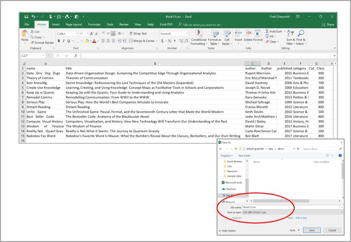
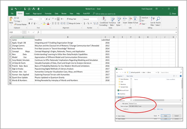
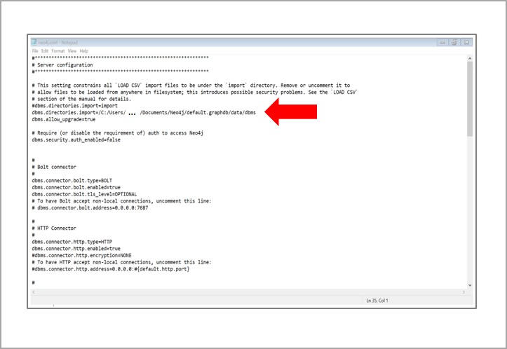
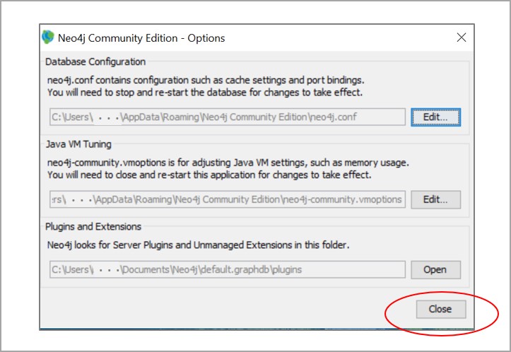
Another alternative is to upload this data as CSV files, as instructed and provided in the following links. This alternative requires file preparation, slight Neo4j configuration modification, additional command use, and also necessitates that you make changes to the ID node/#’s as given in my instructions below. Because this option introduces more complexity, my recommendation is to keep it simple and just follow the steps in the guide.
See Appendix 1, and consult these .csv files (“Book15.csv” and “Review15.csv”) to see what this looks like.
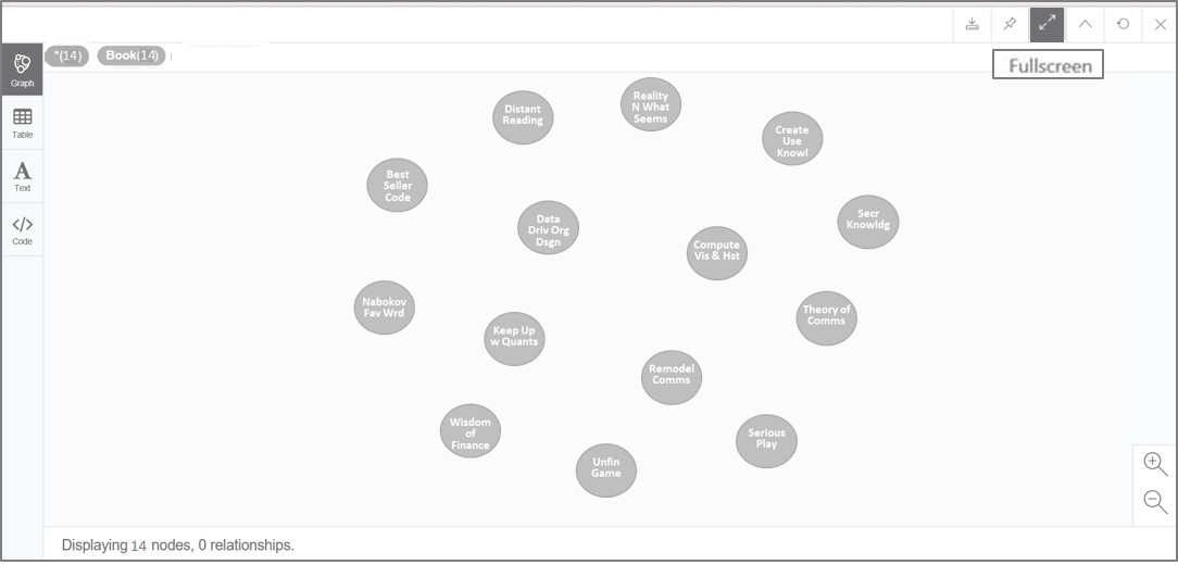
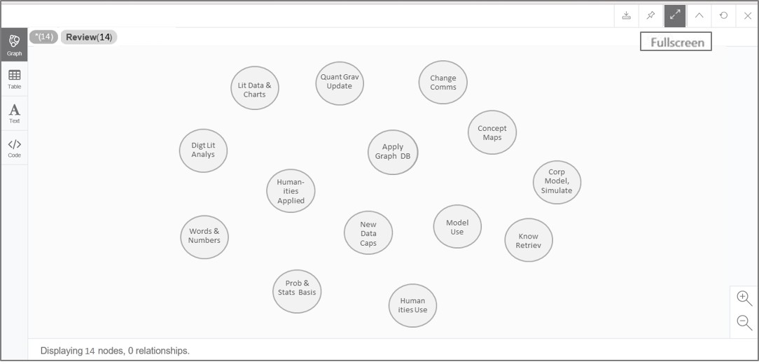
After all the nodes are created, use the following command to get a visual that resembles Figure 5:
| MATCH (n) RETURN n |

Figure 5. All book and review nodes created.
Step 5: Use the command provided below to create a relationship between each of the Sample Booklist and Review Data nodes
Since my Sample Booklist and Review Data refers to a review by me for each book, it is necessary to deliberately create that relationship between those nodes. The Sample Booklist and Review Data in Table 1 only contains the “metadata” or “data about” the book, such as when the book was published and when the review was submitted (completed). However, this data also alludes to information in my review including comments on the content and insights associated with the particular book. For example, the book named “Graph DBs” has a review named “Good/Hard Starter” with a more extended headline reading “Good Graph DB Starter Despite Challenges for Non-Programmers.”
Use with the following command to define and display the book/review relationship as shown in Figure 6.
| MATCH (ya:Review {name: ‘Good/ Hard Starter’}), (xa:Book {name: ‘Graph DBs’}) |
| CREATE (ya)-[r: REVIEW_OF]->(xa) |
| RETURN ya,r,xa |
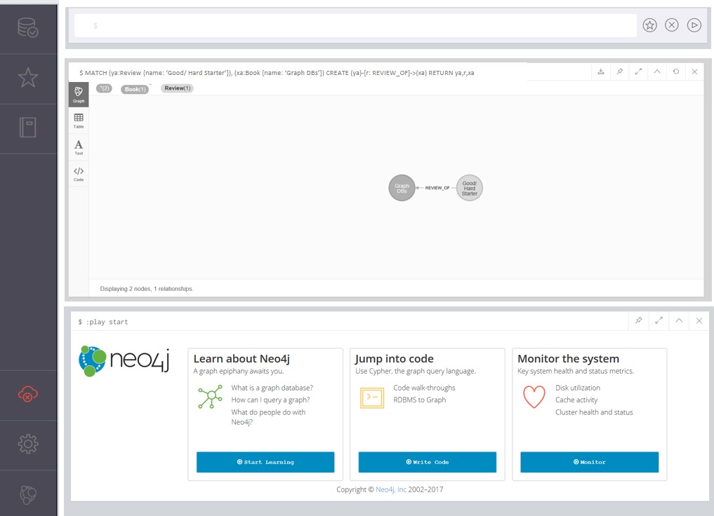
Figure 6. Creating a Review relationship.
Use this command to manually enter booklist and related review relationships until all are included (reminder: see Table 1 again).
When finished with creating booklist and related review relationships, use the display command below again and the resulting visual should approximate the linked nodes shown in Figure 7.
| MATCH (n) RETURN n |
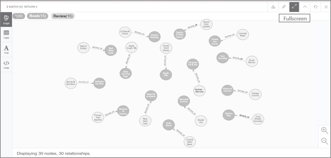
Figure 7. Book and review node relationships.
Step 6: Use of the command below to create a relationship between two Booklist nodes
After the relationships between Sample Booklist and Review Data items have been established, relationships between books should be created. That is, while each book has a review, books have relationships with other books. For instance, the book titled “Graph Databases: New Opportunities for Connected Data, 2nd Edition” is strongly related to the book entitled “Data-driven Organization Design: Sustaining the Competitive Edge Through Organizational Analytics.” From reading these books and writing their reviews where I mention that GDBs were used in organizational modeling, I had a basis to designate a strong relationship between them. Assigning such connections (as I have done with all the books) can lead to visuals and insights made only through analyzing a GDB vs. solely reading the text or going from one reference to another. Follow the command below to establish such a relationship:
| MATCH (xa:Book {name: ‘Graph DBs’}), (xb:Book {name: ‘Data Driv Org Dsgn’}) |
| CREATE (xa)-[r: STRONGLY_RELATED]->(xb) |
| RETURN xa,r,xb |
When finished, the command and the resulting visual of the relationship between book nodes should resemble Figure 8:
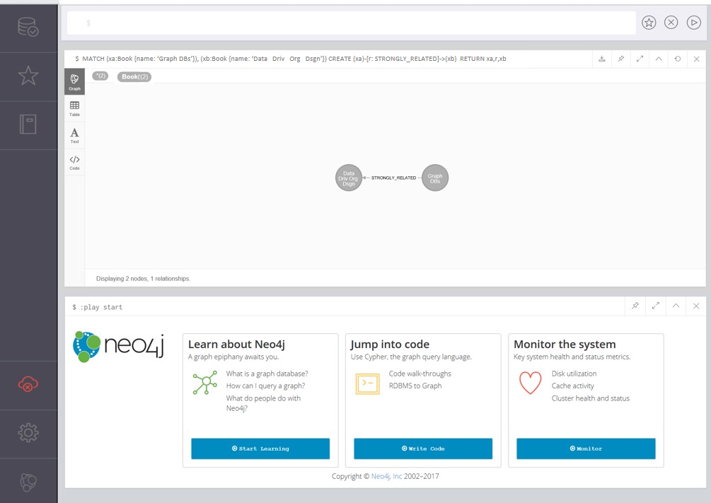
Figure 8. Creating a relationship between book nodes.
It is possible to establish different kinds of relationships among the booklist and related review items with which we are working. The following table shows five types of relationships ranging from books that are strongly related to those that are only somewhat related. This differentiation can help in interpreting the various connections. For example, while “Graph DBs” is Strongly Related to “Data Driv Org Dsgn,” the latter is only Related to “Keep Up w Quants.” See Table 2 where these book relationships are assigned. Look below Table 2 to find the commands needed to create these relationships in the graph data base.
Table 2. Sample book node relationships
|
Order/ID #
|
Book Node Name
|
Book Title
|
Other Book Order/ID #s* | ||||
| Strongly Related | Highly Related | Related | Mostly Related | Somewhat Related | |||
| 1 | Graph DBs | Graph Databases: New Opportunities for Connected Data, 2nd Edition | 3 | 15 | 13 | 21 | |
| 3 | Data Driv Org Dsgn | Data-driven Organization Design: Sustaining the Competitive Edge Through Organizational Analytics | 11 | ||||
| 5 | Theory of Comms | Theories of Communication | 7 | 13 | |||
| 7 | Secr Knowldg | Secret Knowledge: Rediscovering the Lost Techniques of the Old Masters (Expanded) | 23 | 5 | |||
| 9 | Create Use Knowledge | Learning, Creating, and Using Knowledge: Concept Maps as Facilitative Tools in Schools and Corporations | 27 | ||||
| 11 | Keep Up w Quants | Keeping Up with the Quants: Your Guide to Understanding and Using Analytics | 19 | 17 | 3 | ||
| 13 | Remodel Comms | Remodeling Communication: From WWII to the WWW | 5 | 11 | 15 | 23 | |
| 15 | Serious Play | Serious Play: How the World’s Best Companies Simulate to Innovate | 13 | 19 | |||
| 17 | Distant Reading | Distant Reading | 21 | 23 | 11 | ||
| 19 | Unfin Game |
The Unfinished Game: Pascal, Fermat, and the Seventeenth-Century Letter that Made the World Modern
|
11 | 15 | 25 | ||
| 21 | Best Seller Code | The Bestseller Code: Anatomy of the Blockbuster Novel | 17 | ||||
| 23 | Compute Visual History | Computers, Visualization, and History: How New Technology Will Transform Our Understanding of the Past | 13 | 9 | 17 | ||
| 25 | Wisdom of Finance | The Wisdom of Finance | 19 | ||||
| 27 | Reality Not – Quant Grav | Reality is Not What It Seems: The Journey to Quantum Gravity | 23 | 1 | |||
| 29 | Nabokov Fav Word | Nabokov’s Favorite Word Is Mauve: What the Numbers Reveal About the Classics, Bestsellers, and Our Own Writing | 21 | 17 | 11 | 25 | |
*Note also see Table 1 above.
Below are commands that provide ways to create the different types of relationships among books using ID#’s vs. the command by book names used above in Figure 8. Neo4j assigns ID#’s as nodes are created, which is why the entry order matters. Notice how working with the ID#’s is easier than entering the node names. (If you have entered the book and review data using a CSV file, you will likely have to update the Order/ID #’s in Table 2 and also for the commands as well to get the results indicated.)
| MATCH (xa:Book) WHERE ID(xa)=1 |
| MATCH (xb:Book) WHERE ID(xb)=3 |
| CREATE (xa)-[r: STRONGLY_RELATED]->(xb) |
| RETURN xa,r,xb |
| MATCH (xa:Book) WHERE ID(xa)=1 |
| MATCH (xb:Book) WHERE ID(xb)=15 |
| CREATE (xa)-[r: HIGHLY_RELATED]->(xb) |
| RETURN xa,r,xb |
| MATCH (xa:Book) WHERE ID(xa)=3 |
| MATCH (xb:Book) WHERE ID(xb)=11 |
| CREATE (xa)-[r: RELATED]->(xb) |
| RETURN xa,r,xb |
| MATCH (xa:Book) WHERE ID(xa)=1 |
| MATCH (xb:Book) WHERE ID(xb)=13 |
| CREATE (xa)-[r: MOSTLY_RELATED]->(xb) |
| RETURN xa,r,xb |
| MATCH (xa:Book) WHERE ID(xa)=1 |
| MATCH (xb:Book) WHERE ID(xb)=21 |
| CREATE (xa)-[r: SOMEWHAT_RELATED]->(xb) |
| RETURN xa,r,xb |
Repeat the use of the above commands and manually enter the information to create the relationships as listed in Table 2 (Book Node Relationships). Substitute the ID#’s and manually enter, as required, to create all the relationships among the books in the list. When complete, use the following command and the resulting visual should approximate Figure 9, below.
| MATCH (n:Book) RETURN n |
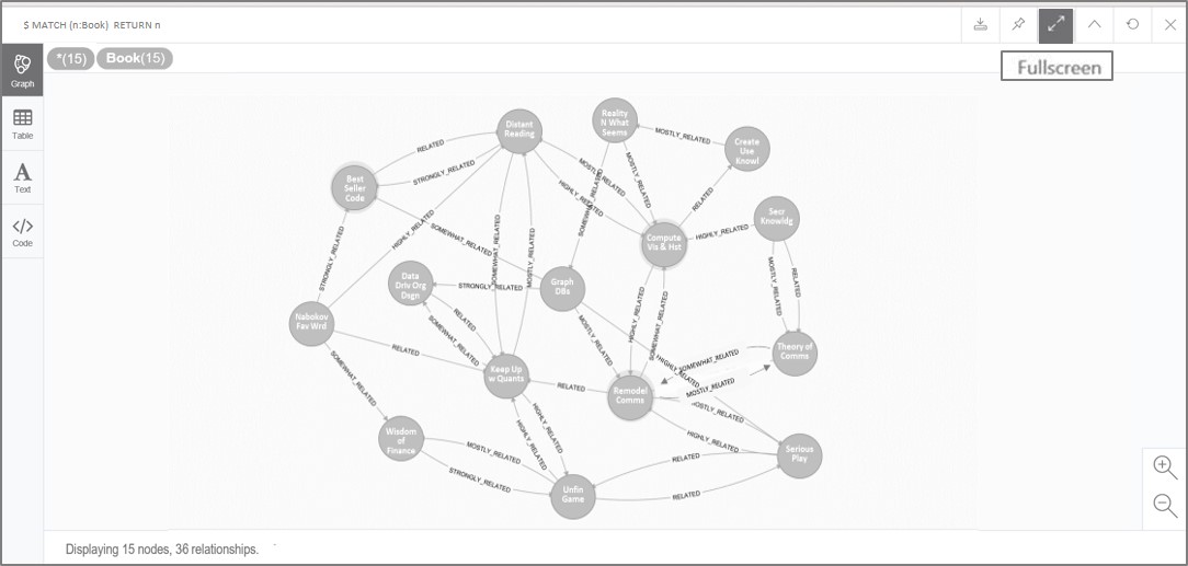
Figure 9. Relationships created between book nodes.
Now the book nodes, review nodes, and their relationships have been created. The pictures above and below provide overviews that cannot be readily gleaned from Table 2 or related text: a simple illustration of the visual benefit of a GDB. Use the following command and the resulting visual should approximate Figure 10 (note how this command uses (n) vs. (n:Book) to get a more expansive display):
| MATCH (n) RETURN n |

Figure 10. Book nodes, review nodes, and relationships created.
Step 7: Refine the graph database by using properties to change labels and corresponding color coding
I assigned colors to book node labels based on the category classification (Cat_Class) property (see Table 1) that allowed me to recognize similarities and differences in the visualization. Use the following commands and assign colors as described below to complete and check the required tasks:
| MATCH (n:Book) WHERE n.Cat_Class =[500] OR n.Cat_Class = [600] |
| REMOVE n:Book |
| SET n:Book_D |
| MATCH (n) WHERE n.Cat_Class =[400] OR n.Cat_Class =[700] OR n.Cat_Class =[800] OR n.Cat_Class =[900] |
| REMOVE n:Book |
| SET n:Book_G |
| MATCH (n:Book) WHERE n.Cat_Class =[100] OR n.Cat_Class =[200] OR n.Cat_Class =[300] |
| REMOVE n:Book |
| SET n:Book_R |
| RETURN n |
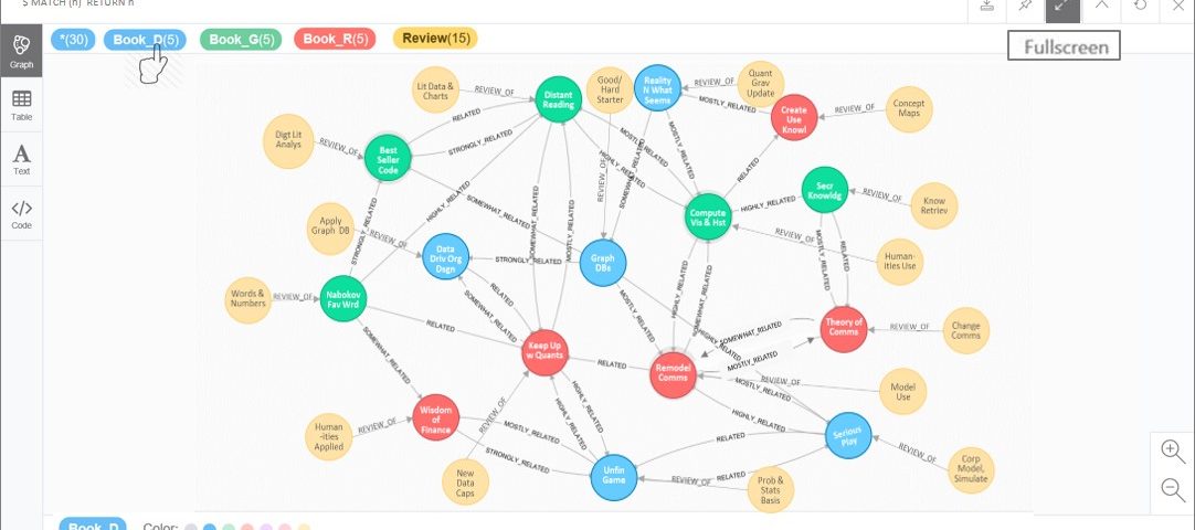
Note in Figure 11 how colors are selected to distinguish node labels. Chose blue (denim) for Book_D, green for Book_G, red for Book_R and yellow or gold for review nodes. In this manner, nine book classifications are subsumed into three supra categories that correspond to the three elements of the classic trivium, i.e. dialectic, rhetoric, and grammar (see Brooks and Mara 2007). Brooks and Mara have proposed that the trivium schema with its concern for knowledge acquisition, application, and critical reflection can be a useful lens in understanding new media, including GDBs. With this scheme and visualization, one can see the interplay at a high level among the three supra category classifications. This graphic can also help show how GDB concepts and display have a relevance in knowledge inquiry.
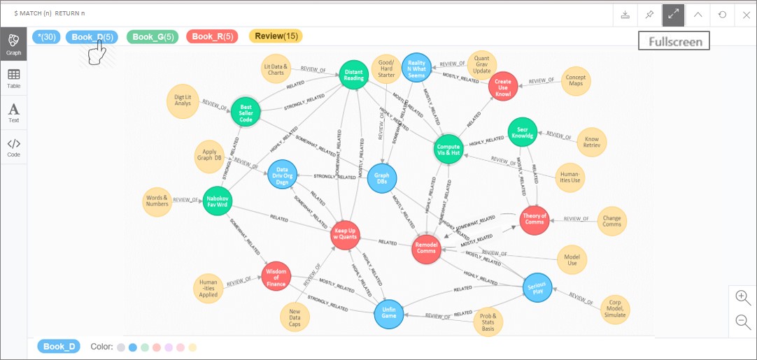
Figure 11. Book nodes and review nodes revised and color coded.
Step 8: Analyze individual book node relationships and other aspects of the GDB
So how do we interpret the GDB once it is constructed? There are numerous ways to analyze GDB nodes and their properties and relationships in addition to visual inspection. One kind of analysis is to count and rank node relationships that, in this instance, could be one indicator of book significance within the sample list.
Use the following command to count and rank book node relationships as shown in Figure 12:
| MATCH (n)-[r]-() |
| RETURN n, COUNT(r) AS REL_COUNT |
| ORDER BY REL_COUNT DESC |
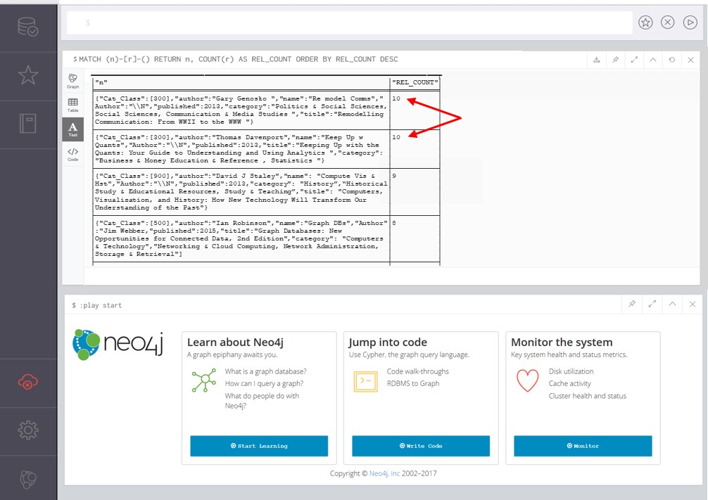
Figure 12. Ranked relationship count by node in text view.
Look specifically at book nodes with the most relationships focusing on the top 4 as indicated in Figure 12. See that there are two Book_R entries with 10 relationships (red arrow), one Book_G and one Book_D entry. These counts provide one way of narrowing in and focusing on the few books that can best provide an initial message to help explain the meaning of this data set.
In order to look at these nodes and their relationships to the highest count books, use the following commands:
| MATCH (a)-[r]-(b) WHERE (a.name = ‘Remodel Comms’) RETURN r, a, b |
The node and relationships returned should appear as in Figure 13. Notice how “Remodel Comms” (Book_R, rhetoric) has 10 connections including the three top count books, across the different classification categories (Book_R, rhetoric; Book_G, grammar; Book_D, dialectic). Because, as the data and graphic indicate, this book has the most relationships overall. With other topped ranked books across categories, we can use such indications in driving the interpretation of our small-scale GDB.
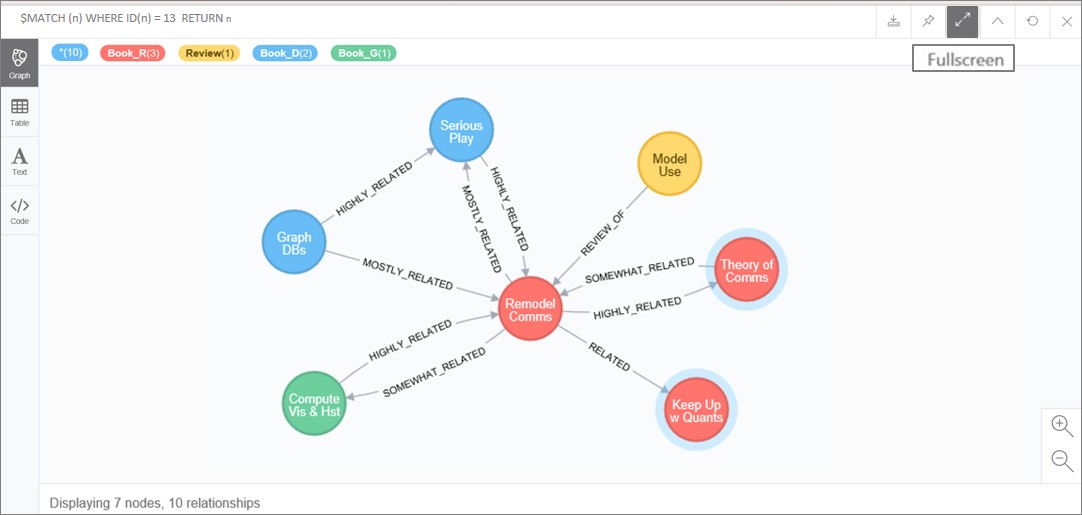
Figure 13. Top ranked Book_R node and related nodes.
Use this same command for the second Book_R node as follows:
| MATCH (a)-[r]-(b) WHERE (a.name = ‘Keep Up w Quants’) RETURN r, a, b |
The node and relationships returned should appear as in Figure 14. Notice that while “Keep Up w Quants” (Book_R) also has 10 varied relationships across different books in the category classification areas, it has only a medium connection to one of the top count books, “Remodel Comms” (Book_R). This data and display seem to indicate that the title be considered a supporting element in deriving the meaning of our GDB.
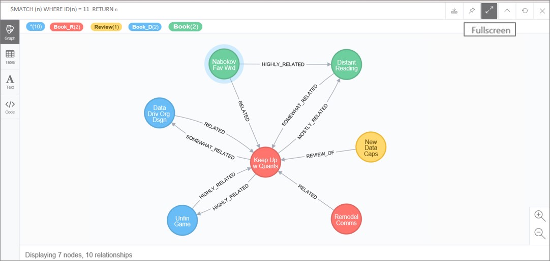
Figure 14. 2nd top ranked Book_R node and related nodes.
Repeat the same command for the Book_G node with nine relationships:
| MATCH (a)-[r]-(b) WHERE (a.name = = ‘Compute Vis & Hst’) RETURN r, a, b |
The node and relationships returned should appear as in Figure 15. Notice again, that “Compute Vis & Hist” (Book_G, grammar) while diverse in its nine relationships has a fairly strong connection to one top count book, “Remodel Comms” (Book_R, rhetoric) also suggests a significant supporting role in determining the meaning of the GDB.
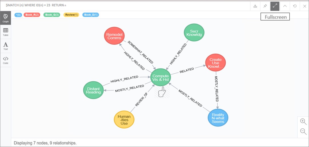
Figure 15. Top ranked Book_G node and related nodes.
Again, use the same command and actions as above for the Book_D node with eight relationships:
| MATC MATCH (a)-[r]-(b) WHERE (a.name = ‘Graph DBs’) RETURN r, a, b |
The node and relationships returned should appear as in Figure 16. As for the previous top count books, the “Graph DBs” (Book_D, dialectic) display is similar, but its eight connections include one with top count “Remodel Comms” (Book_R, rhetoric) and some shared connections with “Serious Play” (Book_D, dialectic) making it a second lead in articulating our GDB’s message.
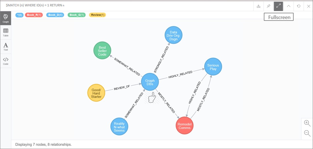
Figure 16. Top ranked Book_D node and related nodes.
For each Figure above recall the top count book nodes, the connections with other book nodes and the observations provided. From this data, one brief interpretation might be that “Remodelling Communication” (and “Keeping Up with the Quants”) using “Graph Databases,” can help enable use of “Computerization, Visualization and History” to advance knowledge inquiry. This information could then be further refined and elaborated using text from the Booklist and Review data as well as related information. Using such an approach for our small-scale GDB could also be used and refreshed as a database is expanded.
To paraphrase Brooke (2009, pages 104-108), the construction of small-scale databases can create possible conditions for the kind of analysis that provides access to trends and patterns that might not otherwise be perceptible.
Step 9: When finished with the above example graph, use the command below to delete this graph, then repeat the above steps with data of your own
At this point, you should be in a position to initiate your own database. Preparing your own small-scale GDB based on your own information will provide you with more practice and will be more meaningful and relevant to your needs.
Caution: Make sure you are ready to delete my GDB data as this information will be gone once the command is entered. However, such deletion will allow you to input your own information and avoid errors or confusion.
| MATCH (n) OPTIONAL MATCH (n)-[r]-() DELETE n, r |
Develop a similar listing of data from an annotated bibliography for a class, dissertation or another resource of your own, as in Tables 1 and 2 above. For instance, for a dissertation, one might substitute references (i.e. books and other sources) and citation information (e.g. key words and pithy characterizations derived from related allusions or quotes) that appear within such a document in place of my Sample Book and Review data. Follow-through, using steps 3 through 8, and see what your GDB can tell you about your own selections. Ask yourself about the number of relationships, the distribution among the classification categories, and other observations. Use the counts to focus on a few key items and form a preliminary interpretation of your GDB. See what insights the visualizations might reveal about the connections or relationships among the sources and their content.
Step 10: Use other learning resources and capabilities to make revisions, add additional data to your GDB, and expand your capabilities
To learn more about GDBs, see other sources (e.g. McKay 2018) and search You Tube (“enter data in Neo4j”) to learn more about projects and inputting data using a CSV file which go beyond our scope herein.
By following these steps, teachers and students can construct a small-scale GDB as a stepping stone to dealing with more complex modeling and analysis of larger scale networked information. This kind of effort can be an individual pursuit, an optional assignment, or a group or class project. Some humanities researchers have begun to use graph databases to develop skills and knowledge among other wider possibilities (see Verhoeven and Burrows 2017).


'Developing a Small-Scale Graph Database: A Ten Step Learning Guide for Beginners' has 4 comments
July 4, 2022 @ 11:02 pm tristinrobin
This Texas-based fast-food chain is well-known for its tasty sandwiches and burgers, and they also offer magnificent breakfast meals everyone loves. Whataburger Breakfast Menu 2022
July 3, 2022 @ 12:46 pm hm4013824
The BitLocker Recovery key will be required if Windows detects an unauthorized attempt to access files. It ensures that your information is protected from breaches.aka.ms/recoverykeyfaq
February 25, 2022 @ 12:08 pm Xeno
Useful, thanks!
May 23, 2021 @ 1:39 pm Carlos Netto
I am 74 years old, engineer and farmer, from Portugal, who worked in development projects and agriculture organization. I use simple RDBMS databases to organize my information. Recently I moved around Graph Databases to seek if it would be possible to use them inquire if is reasonable to investigate matters related to cork quality in a quite large region. I know nothing about code language like Java, Python opr others. I am beginning to read O’Reilly books about this subject.
I am curious because once, about 35 years ago I participated in a rather large project, with a senior engineer wich use statistical software from the Stony Brook University, concerning Numeric Taxonomy (?), and the results where amazing. After such a long time I still consider this last chance to occupy my time.