Introduction
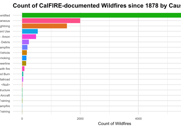
Last Spring one of my students made an important discovery regarding the politics encoded in data about California wildfires. Aishwarya Asthana was examining a dataset published by California’s Department of Forestry and Fire Protection (CalFIRE), documenting the acres burned for each government-recorded wildfire in California from 1878 to 2017. The dataset also included variables such as the fire’s name, when it started and when it was put out, which agency was responsible for it, and the reason it ignited. Asthana was practicing applying techniques for univariate data analysis in R—taking one variable in the dataset and tallying up the number of times each value in that variable appears. Such analyses help to summarize and reveal patterns in the data, prompting questions about why certain values appear more than others.
Tallying up the number of times each distinct wildfire cause appeared in the dataset, Asthana discovered that CalFIRE categorizes each wildfire into one of nineteen distinct cause codes, such as “1—Lightning,” “2—Equipment Use,” “3—Smoking,” and “4—Campfire.” According to the analysis, 184 wildfires were caused by campfires, 1,543 wildfires were caused by lightning, and, in the largest category, 6,367 wildfires were categorized with a “14—Unknown/Unidentified” cause code. The cause codes that appeared the fewest number of times (and thus were attributed to the fewest number of wildfires) were “12—Firefighter Training” and the final code in the list: “19—Illegal Alien Campfire.”
fires %>%
  ggplot(aes(x = reorder(CAUSE,CAUSE,
                     function(x)-length(x)), fill = CAUSE)) +
  geom_bar() +
  labs(title = "Count of CalFIRE-documented Wildfires since 1878 by Cause", x = "Cause", y = "Count of Wildfires") +
  theme_minimal() +
  theme(legend.position = "none",
        plot.title = element_text(size = 12, face = "bold")) +
coord_flip() 
Interpreting the data unreflectively, one might say, “From 1878 to 2017, four California wildfires have been caused by illegal alien campfires—making it the least frequent cause.” Toward the beginning of the quarter in Data Sense and Exploration, many students, particularly those majoring in math and statistics, compose statements like this when asked to draw insights from data analyses. However, in only reading the data on its surface, this statement obscures important cultural and political factors mediating how the data came to be reported in this way. Why are “illegal alien campfires” categorized separately from just “campfires”? Who has stakes in seeing quantitative metrics specific to campfires purportedly ignited by this subgroup of the population—a subgroup that can only be distinctly identified through systems of human classification that are also devised and debated according to diverse political commitments?
While detailing the history of the data’s collection and some potential inconsistencies in how fire perimeters are calculated, the data documentation provided by CalFIRE does not answer questions about the history and stakes of these categories. In other words, it details the provenance of the data but not the provenance of its semantics and classifications. In doing so, it naturalizes the values reported in the data in ways that inadvertently discourage recognition of the human discernment involved in their generation. Yet, even a cursory Web search of the key phrase “illegal alien campfires in California” reveals that attribution of wildfires to undocumented immigrants in California has been used to mobilize political agendas and vilify this population for more than two decades (see, for example, Hill 1996). Discerning the critical import of this data analysis thus demands more than statistical savvy; to assess the quality and significance of this data, an analyst must reflect on their own political and ethical commitments.
Data Sense and Exploration is a course designed to help students reckon with the values reported in a dataset so that they may better judge their integrity. The course is part of a series of undergraduate data studies courses offered in the Science and Technology Studies Program at the University of California Davis, aiming to cultivate student skill in applying critical thinking towards data-oriented environments. Data Sense and Exploration cultivates critical data literacy by walking students through a quarter-long research project contextualizing, exploring, and visualizing a publicly-accessible dataset. We refer to the project as an “ethnography of a dataset,” not only because students examine the diverse cultural forces operating within and through the data, but also because students draw out these forces through immersive, consistent, hands-on engagement with the data, along with reflections on their own positionality as they produce analyses and visualizations. Through a series of labs in which students learn how to quantitatively summarize the features in a dataset in the coding language R (often referred to as a descriptive data analysis), students also practice researching and reflecting on the history of the dataset’s semantics and classification. In doing so, the course encourages students to recognize how the quantitative metrics that they produce reflect not only the way things are in the world, but also how people have chosen to define them. Perhaps, most importantly, the course positions data as always already structured according to diverse biases and thus aims to foster student skill in discerning which biases they should trust and how to responsibly draw meaning from data in spite of them. In this paper, I present how this project is taught in Data Sense and Exploration and some critical findings students made in their projects.
Teaching Critical Data Analysis
With the growth of data science in industry, academic research, and government planning over the past decade, universities across the globe have been investing in the expansion of data-focused course offerings. Many computationally or quantitatively-focused data science courses seek to cultivate student skill in collecting, cleaning, wrangling, modeling, and visualizing data. Simultaneously, high-profile instances of data-driven discrimination, surveillance, and mis-information have pushed universities to also consider how to expand course offerings regarding responsible and ethical data use. Some emerging courses, often taught directly in computer and data science departments, introduce students to frameworks for discerning “right from wrong” in data practice, focusing on individual compliance with rules of conduct at the expense of attention to the broader institutional cultures and contexts that propagate data injustices (Metcalf, Crawford, and Keller 2015). Other emerging courses, informed by scholarship in science and technology studies (STS) and critical data studies (CDS), take a more critical approach, broadening students’ moral reasoning by encouraging them to reflect on the collective values and commitments that shape data and their relationship to law, democracy, and sociality (Metcalf, Crawford, and Keller 2015).
While such courses help students recognize how power operates in and through data infrastructure, a risk is that students will come to see the evaluation of data politics and the auditing of algorithms as a separate activity from data practice. While seeking to cultivate student capacity to foresee the consequences of data work, coursework that divorces reflection from practice end up positioning these assessments as something one does after data analysis in order to evaluate the likelihood of harm and discrimination. Research in critical data studies has indicated that this divide between data science and data ethics pedagogy has rendered it difficult for students to recognize how to incorporate the lessons of data and society into their work (Bates et al. 2020). Thus, Data Sense and Exploration takes a different approach—walking students through a data analysis project while encouraging them, each step of the way, to record field notes on the history and context of their data inputs, the erasures and reductions of narrative that emerge as they clean and summarize the data, and the rhetoric of the visualizations they produce. As a cultural anthropologist, I’ve structured the class to draw from my own training in and engagement with “experimental ethnography” (Clifford and Marcus 1986). Guided by literary, feminist, and postcolonial theory, cultural anthropologists engage experimental ethnographic methods to examine how systems of representation shape subject formation and power. In this sense, Data Sense and Exploration positions data inputs as cultural artifacts, data work as a cultural practice, and ethnography as a method that data scientists can and should apply in their work to mitigate the harm that may arise from them. Importantly, walking students into awareness of the diverse cultural forces operating in and through data helps them more readily recognize opportunities for intervention. Rather than criticizing the values and political commitments that they bring to their work as biasing the data, the course celebrates such judgments when bent toward advancing more equitable representation.
The course is predominantly inspired by literature in data and information infrastructure studies (Bowker et al. 2009). These fields study the cultural and political contexts of data and the infrastructures that support them by interviewing data producers, observing data practitioners, and closely reading data structures. For example, through historical and ethnographic studies of infrastructures for data access, organization, and circulation, the field of data infrastructure studies examines how data is made and how it transforms as it moves between stakeholders and institutions with diverse positionalities and vested interests (Bates, Lin, and Goodale 2016). Critiquing the notion that data can ever be pure or “raw,” this literature argues that all data emerge from sites of active mediation, where diverse epistemic beliefs and political commitments mold what ultimately gets represented and how (Gitelman 2013). Diverting from an outsized focus on data bias, Data Sense and Exploration prompts students to grapple with the “interpretive bases” that frame all data—regardless of whether it has been produced though personal data collection, institutions with strong political proclivities, or automated data collection technologies. In this sense, the course advances what Gray, Gerlitz, and Bounegru (2018) refer to as “data infrastructure literacy” and demonstrates how students can apply critical data studies techniques to critique and improve their own day-to-day data science practice (Neff et al. 2017).
Studying a Dataset Ethnographically
Data Sense and Exploration introduces students to examining a dataset and data practices ethnographically through an extended research project, carried out incrementally through a series of weekly labs.[1] While originally the labs were completed collaboratively in a classroom setting, in the move to remote instruction in Spring 2020, the labs were reformulated as a series of nine R Notebooks, hosted in a public GitHub repository that students clone into their local coding environments to complete. R Notebooks are digital documents, written in the scripting language Markdown, that enable authors to embed chunks of executable R code amidst text, images, and other media. The R Notebooks that I composed for Data Sense and Exploration include text instruction for how to find, analyze, and visualize a rectangular dataset, or a dataset in which values are structured into a series of observations (or rows) each described by a series of variables (or columns). The Notebooks also model how to apply various R functions to analyze a series of example datasets, offer warnings of the various faulty assumptions and statistical pitfalls students may encounter in their own data practice, and demonstrate the critical reflection that students will be expected to engage in as they apply the functions in their own data analysis.
Interspersed throughout the written instruction, example code, and reflections, the Notebooks provide skeleton code for students to fill in as they go about applying what they have learned to a dataset they will examine throughout the course. At the beginning of the course, when many students have no prior programming experience, the skeleton code is quite controlled, asking students to “fill-in-the-blank” with a variable from their own dataset or with a relevant R function.
# Uncomment below and count the distinct values in your unique key. Note that you may need to select multiple variables. If so, separate them by a comma in the select() function.
#n_unique_keys <- _____ %>% select(_____) %>% n_distinct()

# Uncomment below and count the rows in your dataset by filling in your data frame name.
#n_rows <- nrow(_____)

# Uncomment below and then run the code chunk to make sure these values are equal.
# n_unique_keys == n_rowsHowever, as students gain familiarity with the language, each week, they are expected to compose code more independently. Finally, in each Notebook, there are open textboxes, where students record their critical reflections in response to specific prompts.
Teaching this course in the Spring 2020 quarter, I found that the structure provided by the R Notebooks overall was particularly supportive to students who were coding in R for the first time and that, given the examples provided throughout the Notebooks, students exhibited greater depth of reflection in response to prompts. However, without the support of a classroom once we moved online, I also found that novice students struggled more to interpret what the plots they produced in R were actually showing them. Moreover, advanced students were more conservative in their depth of data exploration, closely following the prompts and relying on code templates. In future iterations of the course, I thus intend to spend more synchronous time in class practicing how to quantitatively summarize the results of their analysis. I also plan to add new sections at the end of each Notebook, prompting students to leverage the skills they learned in that Notebook in more creative and free-form data explorations.
Each time I teach the course, individual student projects are structured around a common theme. In the iteration of the course that inspired the project that opens this article, the theme was “social and environmental challenges facing California.” In the most recent iteration of the course, the theme was “social vulnerability in the wake of a pandemic.” In an early lab, I task students with identifying issues warranting public concern related to the theme, devising research questions, and searching for public data that may help answer those questions. Few students entering the course have been taught how to search for public research, let alone how to search for public data. In order to structure their search activity, I task the students with imagining and listing “ideal datasets”—intentionally delineating their topical, geographic, and temporal scope—prior to searching for any data. Examining portals like data.gov, Google’s dataset search, and city and state open data portals, students very rarely find their ideal datasets and realize that they have to restrict their research questions in order to complete the assignment. Grappling with the dearth of public data for addressing complex contemporary questions around equity and social justice provides one of the first eye-opening experiences in the course. A Notebook directive prompts students to reflect on this.
Throughout the following week, I work with groups of students to select datasets from their research that will be the focus of their analysis. This is perhaps one of the most challenging tasks of the course for me as the instructor. While a goal is to introduce students to the knowledge gaps in public data, some public datasets have so little documentation that the kinds of insights students could extrapolate from examinations of their history and content would be considerably limited. Further, not all rectangular datasets are structured in ways that will integrate well with the code templates I provide in the R Notebooks. I grapple with the tension of wanting to expose students to the messiness of real-world data, while also selecting datasets that will work for the assignment.
Once datasets have been assigned, the remainder of the labs provide opportunities for immersive engagement with the dataset. In what follows, I describe a series of concepts (i.e. routines and rituals, semantics, classifications, calculations and narrative, chrono-politics, and geo-politics) around which I have structured each lab, and provide some examples of both the data work that introduced students to these concepts and the critical reflections they were able to make as a result.
Data Routines and Rituals
In one of the earlier labs, students conduct a close reading of their dataset’s documentation—an example of what Geiger and Ribes (2011) refer to as a “trace ethnography.” They note the stakeholders involved in the data’s collection and publication, the processes through which the data was collected, the circumstances under which the data was made public, and the changes in the data’s structure. They also search for news articles and scientific articles citing the dataset to get a sense of how governing bodies have leveraged the data to inform decisions, how social movements have advocated for or against the data’s collection, and how the data has advanced other forms of research. They outline the costs and labor involved in producing and maintaining the data, the formal standards that have informed the data’s structure, and any laws that mandate the data’s collection.
From this exercise, students learn about the diverse “rituals” of data collection and publication (Ribes and Jackson 2013). For instance, studying the North American Breeding Bird Survey (BBS)—a dataset that annually records bird populations along about 4,100 roadside survey routes in the United States and Canada—Tennyson Filcek learned that the data is produced by volunteers skilled in visual and auditory bird identification. After completing training, volunteers drive to an assigned route with a pen, paper, and clipboard and count all of the bird species seen or heard over the course of three minutes along each designated stop on the route. They report the data back to the BBS Office, which aggregates the data and makes them available for public consumption. While these rituals shape how the data get produced, the unruliness of aggregating data collected on different days, by different individuals, under different weather and traffic conditions, and in different parts of the continent has prompted the BBS to implement recommendations and routines to account for disparate conditions. The BBS requires volunteers to complete counts around June, start the route a half-hour before sunrise, and avoid completing counts on foggy, rainy, or windy days. Just as these routines domesticate the data, the heterogeneity of the data’s contexts demands that the data be cared for in particular ways, in turn patterning data collection as a cultural practice. This lab is thus an important precursor to the remaining labs in that it introduces students to the diverse actors and commitments mediating the dataset’s production and affirms that the data could not exist without them.
While I have been impressed with students’ ability to outline details involving the production and structure of the data, I have found that most students rarely look beyond the data documentation for relevant information—often missing critical perspectives from outside commentators (such as researchers, activists, lobbyists, and journalists) that have detailed the consequences of the data’s incompleteness, inconsistencies, inaccuracies, or timeliness for addressing certain kinds of questions. In future iterations of the course, I intend to encourage students to characterize the viewpoints of at least three differently positioned stakeholders in this lab in order to help illustrate how datasets can become contested artifacts.
Data Semantics
In another lab, students import their assigned dataset into the R Notebook and programmatically explore its structure, using the scripting language to determine what makes one observation distinct from the next and what variables are available to describe each observation. As they develop an understanding for what each row of the dataset represents and how columns characterize each row, they refer back to the data documentation to consider how observations and variables are defined in the data (and what these definitions exclude). This focused attention to data semantics invites students to go behind-the-scenes of the observations reported in a dataset and develop a deeper understanding of how its values emerge from judgments regarding “what counts.”
ca_crimes_clearances <- read.csv("https://data-openjustice.doj.ca.gov/sites/default/files/dataset/2019-06/Crimes_and_Clearances_with_Arson-1985-2018.csv")

str(ca_crimes_clearances)
## 'data.frame': 24950 obs. of 69 variables:
## $ Year : int 1985 1985 1985 1985 1985 1985 1985 1985 1985 1985 ...
## $ County : chr "Alameda County" "Alameda County" "Alameda County" "Alameda County" ...
## $ NCICCode : chr "Alameda Co. Sheriff's Department" "Alameda" "Albany" "Berkeley" ...
## $ Violent_sum : int 427 405 101 1164 146 614 671 185 199 6703 ...
## $ Homicide_sum : int 3 7 1 11 0 3 6 0 3 95 ...
## $ ForRape_sum : int 27 15 4 43 5 34 36 12 16 531 ...
## $ Robbery_sum : int 166 220 58 660 82 86 250 29 41 3316 ...
## $ AggAssault_sum : int 231 163 38 450 59 491 379 144 139 2761 ...
## $ Property_sum : int 3964 4486 634 12035 971 6053 6774 2364 2071 36120 ...
## $ Burglary_sum : int 1483 989 161 2930 205 1786 1693 614 481 11846 ...
## $ VehicleTheft_sum : int 353 260 55 869 102 350 471 144 74 3408 ...
## $ LTtotal_sum : int 2128 3237 418 8236 664 3917 4610 1606 1516 20866 ...
## $ ViolentClr_sum : int 122 205 58 559 19 390 419 146 135 2909 ...
## $ HomicideClr_sum : int 4 7 1 4 0 2 4 0 1 62 ...
## $ ForRapeClr_sum : int 6 8 3 32 0 16 20 6 8 319 ...
## $ RobberyClr_sum : int 32 67 23 198 4 27 80 21 16 880 ...
## $ AggAssaultClr_sum : int 80 123 31 325 15 345 315 119 110 1648 ...
## $ PropertyClr_sum : int 409 889 166 1954 36 1403 1344 422 657 5472 ...
## $ BurglaryClr_sum : int 124 88 62 397 9 424 182 126 108 1051 ...
## $ VehicleTheftClr_sum: int 7 62 16 177 8 91 63 35 38 911 ...
## $ LTtotalClr_sum : int 278 739 88 1380 19 888 1099 261 511 3510 ...
## $ TotalStructural_sum: int 22 23 2 72 0 37 17 17 7 287 ...
## $ TotalMobile_sum : int 6 4 0 23 1 26 18 9 3 166 ...
## $ TotalOther_sum : int 3 5 0 5 0 61 21 64 2 22 ...
## $ GrandTotal_sum : int 31 32 2 100 1 124 56 90 12 475 ...
## $ GrandTotClr_sum : int 11 7 1 20 0 14 7 2 2 71 ...
## $ RAPact_sum : int 22 9 2 31 4 21 25 9 15 451 ...
## $ ARAPact_sum : int 5 6 2 12 1 13 11 3 1 80 ...
## $ FROBact_sum : int 77 56 23 242 35 38 136 13 22 1120 ...
## $ KROBact_sum : int 22 23 2 71 10 7 43 3 4 264 ...
## $ OROBact_sum : int 3 11 2 43 11 3 7 1 1 107 ...
## $ SROBact_sum : int 64 130 31 304 26 38 64 12 14 1825 ...
## $ HROBnao_sum : int 59 136 26 351 56 32 116 3 0 1676 ...
## $ CHROBnao_sum : int 38 48 15 150 9 21 43 4 13 253 ...
## $ GROBnao_sum : int 23 2 1 0 2 7 43 6 9 83 ...
## $ CROBnao_sum : int 32 2 2 0 0 8 21 2 2 46 ...
## $ RROBnao_sum : int 11 20 6 47 14 9 19 3 2 306 ...
## $ BROBnao_sum : int 3 2 3 21 0 2 6 0 3 37 ...
## $ MROBnao_sum : int 0 10 5 91 1 7 2 11 12 915 ...
## $ FASSact_sum : int 25 16 3 47 6 47 43 10 26 492 ...
## $ KASSact_sum : int 27 30 2 103 8 38 55 13 21 253 ...
## $ OASSact_sum : int 111 90 10 224 9 120 208 29 43 396 ...
## $ HASSact_sum : int 68 27 23 76 36 286 73 92 49 1620 ...
## $ FEBURact_Sum : int 1177 747 85 2040 161 1080 1128 341 352 9011 ...
## $ UBURact_sum : int 306 242 76 890 44 706 565 273 129 2835 ...
## $ RESDBUR_sum : int 1129 637 100 2015 89 1147 1154 411 274 8487 ...
## $ RNBURnao_sum : int 206 175 33 597 32 292 295 100 44 2114 ...
## $ RDBURnao_sum : int 599 195 44 1418 26 485 532 163 103 5922 ...
## $ RUBURnao_sum : int 324 267 23 0 31 370 327 148 127 451 ...
## $ NRESBUR_sum : int 354 352 61 915 116 639 539 203 207 3359 ...
## $ NNBURnao_sum : int 216 119 32 224 44 274 238 104 43 1397 ...
## $ NDBURnao_sum : int 47 46 21 691 14 110 45 34 26 1715 ...
## $ NUBURnao_sum : int 91 187 8 0 58 255 256 65 138 247 ...
## $ MVTact_sum : int 233 187 42 559 85 219 326 76 56 2711 ...
## $ TMVTact_sum : int 56 33 4 55 9 71 88 40 9 121 ...
## $ OMVTact_sum : int 64 40 9 255 8 60 57 28 9 576 ...
## $ PPLARnao_sum : int 5 31 26 133 5 10 1 4 3 399 ...
## $ PSLARnao_sum : int 60 20 4 163 4 14 20 6 3 251 ...
## $ SLLARnao_sum : int 289 664 40 1277 1 704 1058 106 435 1123 ...
## $ MVLARnao_sum : int 930 538 147 3153 207 1136 753 561 241 8757 ...
## $ MVPLARnao_sum : int 109 673 62 508 153 446 1272 155 252 901 ...
## $ BILARnao_sum : int 205 516 39 611 16 360 334 276 151 349 ...
## $ FBLARnao_sum : int 44 183 46 1877 85 493 417 187 281 4961 ...
## $ COMLARnao_sum : int 11 53 17 18 24 27 59 7 2 70 ...
## $ AOLARnao_sum : int 475 559 37 496 169 727 696 304 148 4055 ...
## $ LT400nao_sum : int 753 540 84 533 217 937 1089 370 235 976 ...
## $ LT200400nao_sum : int 437 622 68 636 122 607 802 299 262 2430 ...
## $ LT50200nao_sum : int 440 916 128 2793 161 1012 1102 453 464 4206 ...
## $ LT50nao_sum : int 498 1159 138 4274 164 1361 1617 484 555 13254 ...For instance, studying aggregated totals of crimes and clearances for each law enforcement agency in California in each year from 1985 to 2017, Simarpreet Singh noted how the definition of a crime gets mediated by rules in the US Federal Bureau of Investigation (FBI)’s Uniform Crime Reporting Program (UCR)—the primary source of statistics on crime rates in the US. Singh learned that one such rule, known as the hierarchy rule, states that if multiple offenses occur in the context of a single crime incident, for the purposes of crime reporting, the law enforcement agency classifies the crime only according to the most serious offense. In descending order, these classifications include 1. Criminal Homicide 2. Criminal Sexual Assault 3. Robbery 4. Aggravated Battery/Aggravated Assault 5. Burglary 6. Theft 7. Motor Vehicle Theft 8. Arson. This means that in the resulting data, for incidents where multiple offenses occurred, certain classes of crime are likely to be underrepresented in the counts.
Sidhu also acknowledged how counts for individual offense types get mediated by official definitions. A change in the FBI’s definition of “forcible rape” (including only female victims) to “rape” (focused on whether there had been consent instead of whether there had been physical force) in 2014 led to an increase in the number of rapes reported in the data from that year on. From 1927 (when the original definition was documented) up until this change, male victims of rape had been left out of official statistics, and often rapes that did not involve explicit physical force (such as drug-facilitated rapes) went uncounted. Such changes come about, not in a vacuum, but in the wake of shifting norms and political stakes to produce certain types of quantitative information (Martin and Lynch 2009). By encouraging students to explore these definitions, this lab has been particularly effective in getting students to reflect not only on what counts and measures of cultural phenomena indicate, but also on the cultural underpinnings of all counts and measures.
Data Classifications
In the following lab, students programmatically explore how values get categorized in the dataset, along with the frequency with which each observation falls into each category. To do so, they select categorical variables in the dataset and produce bar plots that display the distributions of values in that variable. Studying a US Environmental Protection Agency (EPA) dataset that reported the daily air quality index (AQI) of each county in the US in 2019, Farhat Bin Aznan created a bar plot that displayed the number of counties that fell into each of the following air quality categories on January 1, 2019: Good, Moderate, Unhealthy for Sensitive Populations, Unhealthy, Very Unhealthy, and Hazardous.
aqi$category <- factor(aqi$category, levels = c("Good", "Moderate", "Unhealthy for Sensitive Groups", "Unhealthy", "Very Unhealthy", "Hazardous"))

aqi %>%
  filter(date == "2019-01-01") %>%
  ggplot(aes(x = category, fill = category)) +
  geom_bar() +
  labs(title = "Count of Counties in the US by Reported AQI Category on January 1, 2019", subtitle = "Note that not all US counties reported their AQI on this date", x = "AQI Category", y = "Count of Counties") +
  theme_minimal() +
  theme(legend.position = "none",
        plot.title = element_text(size = 12, face = "bold")) +
  scale_fill_brewer(palette="RdYlGn", direction=-1)
Studying the US Department of Education’s Scorecard dataset, which documents statistics on student completion, debt, and demographics for each college and university in the US, Maxim Chiao created a bar plot that showed the number of universities that fell into each of the following ownership categories: Private, Public, Non-profit.
scorecard %>%
  mutate(CONTROL_CAT = ifelse(CONTROL == 1, "Public",
                          ifelse(CONTROL== 2, "Private nonprofit",
                                 ifelse(CONTROL == 3, "Private for-profit", NA)))) %>%
           ggplot(aes(x = CONTROL_CAT, fill = CONTROL_CAT)) +
           geom_bar() +
           labs(title ="Count of Colleges and Universities in the US by Ownership Model, 2018-2019", x = "Ownership Model", y = "Count of Colleges and Universities") +
           theme_minimal() +
           theme(legend.position = "none",
                 plot.title = element_text(size = 12, face = "bold"))
I first ask students to interpret what they see in the plot. Which categories are more represented in the data, and why might that be the case? I then ask students to reflect on why the categories are divided the way that they are, how the categorical divisions reflect a particular cultural moment, and to consider values that may not fit neatly into the identified categories. As it turns out, the AQI categories in the EPA’s dataset are specific to the US and do not easily translate to the measured AQIs in other countries, where for a variety of reasons, different pollutants are taken into consideration when measuring air quality (Plaia and Ruggieri 2011). The ownership models categorized in the Scorecard dataset gloss over the nuance of quasi-private universities in the US such as the University of Pittsburgh and other universities in Pennsylvania’s Commonwealth System of Higher Education.
For some students, this Notebook was particularly effective in encouraging reflection on how all categories emerge in particular contexts to delimit insight in particular ways (Bowker and Star 1999). For example, air pollution does not know county borders, yet, as Victoria McJunkin pointed out in her labs, the EPA reports one AQI for each county based on a value reported from one air monitor that can only detect pollution within a delimited radius. AQI is also reported on a daily basis in the dataset, yet for certain pollutants in the US, pollution concentrations are monitored on an hourly basis, averaged over a series of hours, and then the highest average is taken as the daily AQI. The choice to classify AQI by county and day then is not neutral, but instead has considerable implications for how we come to understand who experiences air pollution and when.
Still, I found that, in this lab, other students struggled to confront their own assumptions about categories they consider to be neutral. For instance, many students categorizing their data by state in the US suggested that there were no cultural forces underlying these categories because states are “standard” ways of dividing the country. In doing so, they missed critical opportunities to reflect on the politics behind how state boundaries get drawn and which people and places get excluded from consideration when relying on this bureaucratic schema to classify data. Going forward, to help students place even “standard” categories in a cultural context, I intend to prompt students to produce a brief timeline outlining how the categories emerged (both institutionally and discursively) and then to identify at least one thing that remains “residual” (Star and Bowker 2007) to the categories.
Data Calculations and Narrative
The next lab prompts students to acknowledge the judgment calls they make in performing calculations with data, including how these choices shape the narrative the data ultimately conveys. Selecting a variable that represents a count or a measure of something in their data, students measure the central tendency of the variable—taking an average across the variable by calculating the mean and the median value. Noting that they are summarizing a value across a set of numbers, I remind students that such measures should only be taken across “similar” observations, which may require first filtering the data to a specific set of observations or performing the calculations across grouped observations. The Notebook instructions prompt students to apply such filters and then reflect on how they set their criteria for similarity. Where do they draw the line between relevant or irrelevant, similar or dissimilar? What narratives do these choices bring to the fore, and what do they exclude from consideration?
For instance, studying a dataset documenting changes in eligibility policies for the US Supplemental Nutrition Assistance Program (SNAP) by state since 1995, Janelle Marie Salanga sought to calculate the average spending on SNAP outreach across geographies in the US and over time. Noting that we could expect there to be differences in state spending on outreach due to differences in population, state fiscal politics, and food accessibility, Salanga decided to group the observations by state before calculating the average spending across time. Noting that the passing of the American Recovery and Reinvestment Act of 2009 considerably expanded SNAP benefits to eligible families, Salanga decided to filter the data to only consider outreach spending in the 2009 fiscal year through the 2015 fiscal year. Through this analysis, Salanga found California to have, on average, spent the most on SNAP outreach in the designated fiscal years, while several states spent nothing.
snap %>%
  filter(month(yearmonth) == 10 & year(yearmonth) %in% 2009:2015) %>% #Outreach spending is reported annually, but this dataset is reported monthly, so we filter to the observations on the first month of each fiscal year (October)
  group_by(statename) %>%
  summarize(median_outreach = median(outreach * 1000, na.rm = TRUE),
            num_observations = n(),
            missing_observations = paste(as.character(sum(is.na(outreach)/n()*100)), "%"),
            .groups = 'drop') %>%
arrange(desc(median_outreach))| statename | median_outreach | num_observations | missing_observations |
|---|---|---|---|
| California | 1129009.3990 | 7 | 0 % |
| New York | 469595.8557 | 7 | 0 % |
| Texas | 422051.5137 | 7 | 0 % |
| Washington | 273772.9187 | 7 | 0 % |
| Minnesota | 261750.3357 | 7 | 0 % |
| Arizona | 222941.9250 | 7 | 0 % |
| Nevada | 217808.7463 | 7 | 0 % |
| Illinois | 195910.5835 | 7 | 0 % |
| Connecticut | 184327.4231 | 7 | 0 % |
| Georgia | 173554.0009 | 7 | 0 % |
| Pennsylvania | 153474.7467 | 7 | 0 % |
| South Carolina | 126414.4135 | 7 | 0 % |
| Ohio | 125664.8331 | 7 | 0 % |
| Rhode Island | 99755.1651 | 7 | 0 % |
| Tennessee | 98411.3388 | 7 | 0 % |
| Massachusetts | 97360.4965 | 7 | 0 % |
| Wisconsin | 87527.9999 | 7 | 0 % |
| Maryland | 81700.3326 | 7 | 0 % |
| Vermont | 69279.2511 | 7 | 0 % |
| North Carolina | 62904.8309 | 7 | 0 % |
| Indiana | 58047.9164 | 7 | 0 % |
| Oregon | 57951.0803 | 7 | 0 % |
| Michigan | 53415.1688 | 7 | 0 % |
| Florida | 37726.1696 | 7 | 0 % |
| Hawaii | 29516.3345 | 7 | 0 % |
| New Jersey | 23496.2501 | 7 | 0 % |
| Missouri | 23289.1655 | 7 | 0 % |
| Louisiana | 20072.0005 | 7 | 0 % |
| Colorado | 19113.8344 | 7 | 0 % |
| Iowa | 18428.9169 | 7 | 0 % |
| Virginia | 15404.6669 | 7 | 0 % |
| Delaware | 14571.0001 | 7 | 0 % |
| Alabama | 11048.8329 | 7 | 0 % |
| District of Columbia | 9289.5832 | 7 | 0 % |
| Kansas | 8812.2501 | 7 | 0 % |
| North Dakota | 8465.0002 | 7 | 0 % |
| Mississippi | 4869.0000 | 7 | 0 % |
| Alaska | 3199.3332 | 7 | 0 % |
| Arkansas | 3075.0833 | 7 | 0 % |
| Nebraska | 217.1667 | 7 | 0 % |
| Idaho | 0.0000 | 7 | 0 % |
| Kentucky | 0.0000 | 7 | 0 % |
| Maine | 0.0000 | 7 | 0 % |
| Montana | 0.0000 | 7 | 0 % |
| New Hampshire | 0.0000 | 7 | 0 % |
| New Mexico | 0.0000 | 7 | 0 % |
| Oklahoma | 0.0000 | 7 | 0 % |
| South Dakota | 0.0000 | 7 | 0 % |
| Utah | 0.0000 | 7 | 0 % |
| West Virginia | 0.0000 | 7 | 0 % |
| Wyoming | 0.0000 | 7 | 0 % |
The students then consider how their measures may be reductionist—that is, how the summarized values erase the complexity of certain narratives. For instance, Salanga went on to plot a series of boxplots that displayed the dispersion of outreach spending across fiscal years for each state from 2009 to 2015. She found that, while outreach spending had been fairly consistent in several states across these years, in other states there had been a difference in several hundred thousand dollars from the fiscal year with the maximum outreach spending to the year with the minimum.
snap %>%
  filter(month(yearmonth) == 10 & year(yearmonth) %in% 2009:2015) %>%
  ggplot(aes(x = statename, y = outreach * 1000)) +
  geom_boxplot() +
  coord_flip() +
  labs(title = "Distribution of Annual SNAP Outreach Spending per State from 2009 to 2015", x = "State", y = "Outreach Spending") +
  scale_y_continuous(labels = scales::comma) +
  theme_minimal() +
theme(plot.title = element_text(size = 12, face = "bold")) 
This nuanced story of variations in spending over time gets obfuscated when relying on a measure of central tendency alone to summarize the values.
This lab has been effective in getting students to recognize data work as a cultural practice that involves active discernment. Still, I have noticed that some students complete this lab feeling uncomfortable with the idea that the choices they make in data work may be framed, at least in part, by their own political and ethical commitments. In other words, in their reflections, some students describe their efforts to divorce their own views from their decision-making: they express concern that their choices may be biasing the analysis in ways that invalidate the results. To help them further grapple with the judgment calls that frame all data analyses (and especially the calls that they individually make when choosing how to filter, sort, group, and visualize the data), the next time I run the course I plan to ask students to explicitly characterize their own standpoint in relation to the analysis and reflect on how their unique positionality both influences and delimits the questions they ask, the filters they apply, and the plots they produce.
Data Chrono-Politics and Geo-Politics
In a subsequent lab, I encourage students to situate their datasets in a particular temporal and geographic context in order to consider how time and place impact the values recorded. Students first segment their data by a geographic variable or a date variable to assess how the calculations and plots vary across geographies and time. They then characterize, not only how and why there may be differences in the phenomena represented in the data across these landscapes and timescapes, but also how and why there may be differences in the data’s generation.
For instance, in Spring 2020, a group of students studied a dataset documenting the number of calls related to domestic violence received each month to each law enforcement agency in California.
dom_violence_calls %>%
  ggplot(aes(x = YEAR_MONTH, y = TOTAL_CALLS, group = 1)) +
  stat_summary(geom = "line", fun = "sum") +
  facet_wrap(~COUNTY) +
  labs(title = "Domestic Violence Calls to California Law Enforcement Agencies by County", x = "Month and Year", y = "Total Calls") +
  theme_minimal() +
  theme(plot.title = element_text(size = 12, face = "bold"),
        axis.text.x = element_text(size = 5, angle = 90, hjust = 1),
        strip.text.x = element_text(size = 6))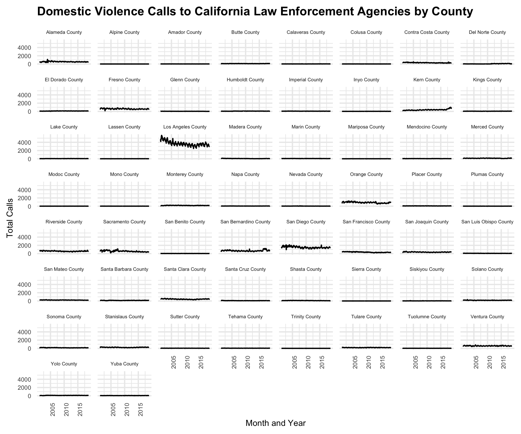
One student, Laura Cruz, noted how more calls may be reported in certain counties not only because domestic violence may be more prevalent or because those counties had a higher or denser population, but also due to different cultures of police intervention in different communities. Trust in law enforcement may vary across California communities, impacting which populations feel comfortable calling their law enforcement agencies to report any issues. This creates a paradox in which the counts of calls related to domestic violence can be higher in communities that have done a better job responding to them.
Describing how the values reported may change over time, Hipolito Angel Cerros further noted that cultural norms around domestic violence have changed over time for certain social groups. As a result of this cultural change, certain communities may be more likely to call law enforcement agencies regarding domestic violence in 2020 than they were a decade ago, while other communities may be less likely to call.
This was one of the course’s more successful labs, which helped students discern the ways in which data are products of the cultural contexts of their production. Dividing the data temporally and geographically helped affirm the dictum that “all data are local” (Loukissas 2019)—that data emerge from meaning-making practices that are never completely stable. Leveraging data visualization techniques to situate data in particular times and contexts demonstrated how, when aggregated across time and place, datasets can come to tell multiple stories from multiple perspectives at once. This called on students, in their role as data practitioners, to convey data results with more care and nuance.
Conclusion
Ethnographically analyzing a dataset can draw to the fore insights about how various people and communities perceive difference and belonging, how people represent complex ideas numerically, and how they prioritize certain forms of knowledge over others. Programmatically exploring a dataset’s structure, schemas, and contexts helped students see datasets not just as a series of observations, counts, and measurements about their communities, but also as cultural objects, conveying meaning in ways that foreground some issues while eclipsing others. The project also helped students see data science as a practice that is always already political, as opposed to something that can potentially become politicized when placed into the wrong hands or leveraged in the wrong ways. Notably, the project helped students cultivate these insights by integrating a computational practice with critical reflection, highlighting how they can incorporate social awareness and critique into their work. Still, the course content could be strengthened to encourage more critical examinations of categories students consider to be standard, and to better connect their choices in data analysis with their own political and ethical commitments.
Notably, there is great risk to calling attention to just how messy public data is, especially in a political moment in the US where a growing culture of denialism is undermining the credibility of evidence-based research. I encourage students to see themselves as data auditors and their work in the course as responsible data stewardship, and on several occasions, we have worked together to compose emails to data publishers describing discrepancies we have found in the datasets. In this sense, rather than disparaging data for its incompleteness, inconsistencies, or biases, the project encourages students to rethink their role as critical data practitioners, responsible for considering when and how to advocate for making datasets and data analysis more comprehensive, honest, and equitable.